Conventions:
Note: This post is for comparing the differences and understanding the similarities of various model-free prediction algorithms for (deep) reinforcement learning (especially with function approximations). Red colored fonts indicates the comparable differences (if applicable) from the preceding equation/algorithm. Some of the details may be left out for brievity. Please refer to Sutton & Barto, 2017 and the cited papers for completeness.
equivalently, \(\begin{align}g_{t,\mathbf w_t}^{(n)}= \sum_{i=1}^n \gamma^{i-1} * r_{t+i} + \gamma^{n} * \hat V(s_{t+n},\mathbf w_t)\end{align}\)
The $\lambda-return$, $g_{t,\mathbf{w_t}}^{\lambda}$ combines all n-step (from the current time step) returns using $\lambda^{n-1}$ as the weights for each of the n-step returns. $(1-\lambda)$ is the normalizing term so that, $(1-\lambda) \sum_{n=1}^{\infty}\lambda^{n-1}=1$. Visually, it makes intuitive sense:
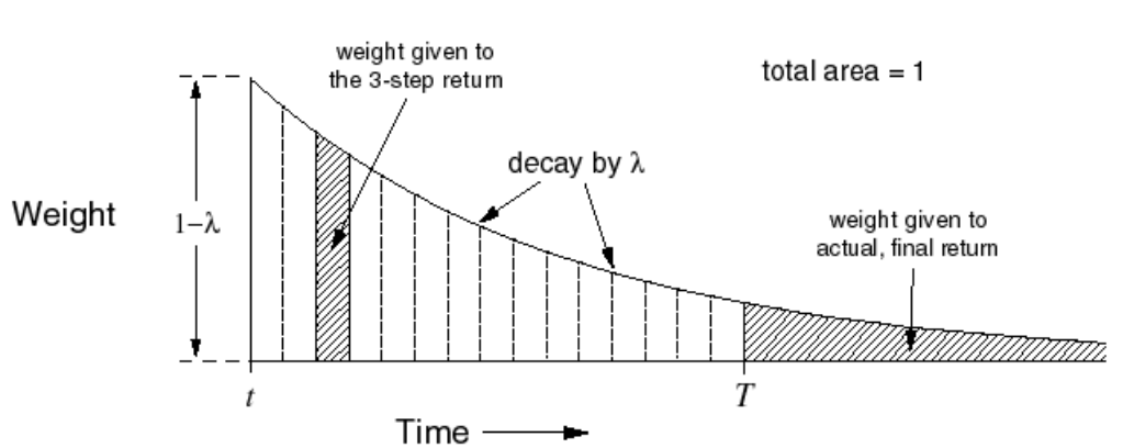
Let T be the time step at which a terminal state is reached which marks the end of an episode. Therefore, the number of steps that can be taken from the current time step t until the end of the episode is $T-t$ .
\[\begin{align}{\displaystyle g_{t,\mathbf{w_t}}^{(\lambda)}= (1-\lambda) \sum_{n=1}^{\color{red}{T-t}}\lambda^{n-1}g_{t,\mathbf{w_t}}^{(n)}}\end{align}\](Question: Is the normalizing factor of $(1-\lambda)$ still valid? If n goes till $\infty$, summation of $\lambda^{n-1}$ approaches $\frac{1}{1-r}$. For the summation still $T-t$, the term comes to $\frac{1-\lambda^{T-t-1}}{1-\lambda}$. Is the term $1-\lambda$ still the normalizing factor? )
We can pull out the last term from this summation and write it as:
\[\begin{align}g_{t,\mathbf{w_t}}^{(\lambda)}= \underbrace{(1-\lambda) \sum_{n=1}^{\color{red}{T-t-1}}\lambda^{n-1}g_{t,\mathbf{w_t}}^{(n)}}_{\text{For steps until the end of episode}} + \underbrace{\color{red}{\lambda^{T-t-1}g_{t,\mathbf{w_t}}^{(T-t)}}}_{\text{For step(s) after end of episode}}\end{align}\]By the definition of an episodic MDP, after the end of an episode (i.e after a terminal state is reached), there is nothing for an agnet to do. By observation, the last n-step return, ${\color{green}{\lambda^{T-t-1}g_{t,\mathbf{w_t}}^{T-t}}}$ is $\color{green}{equal}$ to the full return, $\color{green}{g_{t,\mathbf{w_t}}}$ of the episode.
\[\begin{align}g_{t,\mathbf{w_t}}^{(T-t)}=\sum_{i=1}^{T-t}\gamma^{i-1}r_{t+i}=g_{t,\mathbf{w_t}}\end{align}\nonumber\]Off-line^1 TD($\lambda$) is equivalent to the (off-line) $\lambda-return$ algorithm Sutton & Barto; 1998,Sutton; 1988. However, online^2 TD($\lambda$) is only approximately equal to the online $\lambda-return$ algorithm. Seijen & Sutton; 2014 proposed the use of truncated $\lambda-return$ that truncates the $\lambda-return$ at a specific timestep $t’$ to pave way for the strict-online forward view algorithm.
\[\begin{align}g_{t,\mathbf w_t}^{\color{red}{\lambda|t'}}= (1-\lambda) \sum_{n=1}^{\color{red}{t'-t-1}} \lambda^{n-1}g_{t,\mathbf {w_{\color{red}{t+n-1}}}}^{(n)}+\lambda^{\color{red}{t'-t-1}} g_{t,\mathbf w_{\color{red}{t'-t}}}^{\color{red}{t'-t}}\end{align}\]Updates are accumulated after every step within an episode but applied in batch at the end of the episode.
Updates are applied online at each time step within an episode
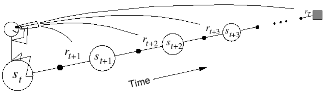
For each visited state, look forward in time to all the subsequent rewards and the sates visited to determine its update.
At time step $t+1$, the error at timestep $t$ is used to adjust the estimate of $V(s_t,\mathbf{w_t})$ through the following weight (of the State-value function approximator) update:
TD(0) updates the weights using one-step return, $r_{t+1} + \gamma * \hat V(s_{t+1},\mathbf w_t)$. This update depends on the immediate reward, $r_{t}$ and the current (at time step $t$) approximation of the value of the next state, $\hat V(s_t,\mathbf w_t)$.
or \(\begin{align}\Delta \mathbf{w_{t+1}}=\alpha * \delta_t*\mathbf e_{t,\mathbf w_t}(s_t)\end{align}\)
where,
\[\mathbf e_{t,\mathbf{w_t}} (s_t)= \gamma \lambda e_{t-1,\mathbf w_t}(s_t) +\nabla_{\mathbf w_t}\hat V(s_t, \mathbf w_t)\]and \(\begin{align}\delta_t= r_{t+1} + \gamma * \hat V(s_{t+1},\mathbf{w_t})-\hat V(s_t, \mathbf w_t)\end{align}\)
True online TD($\lambda$) forms the backward view of the truncated $\lambda-return$ algorithm. Like the vanilla TD($\lambda$), it updates the weights proportional to a decaying eligibility trace.
\[\begin{align}\Delta \mathbf{w_{t+1}}=\alpha * [ r_{t+1} + \gamma * \hat V(s_{t+1},\mathbf{w_t})-\hat V(s_t, \mathbf w_t)]*\mathbf e_{t,\mathbf w_t}(s_t)\color{red}{+\alpha_t[\hat V(s_t,\mathbf{w_{t-1}})-\hat V(s_t,\mathbf{w_{t}})]\nabla_{\mathbf w_t}\hat V(s_t, \mathbf w_t)}\end{align}\]or \(\begin{align}\Delta \mathbf{w_{t+1}}=\alpha * \delta_t*\mathbf e_{t,\mathbf w_t}(s_t)\color{red}{+\alpha_t[\hat V(s_t,\mathbf{w_{t-1}})-\hat V(s_t,\mathbf{w_{t}})]\nabla_{\mathbf w_t}\hat V(s_t, \mathbf w_t)}\end{align}\)
where,
\[\begin{align}\mathbf e_{t,\mathbf{w_t}} (s_t)= \gamma \lambda e_{t-1,\mathbf w_t}(s_t) +\nabla_{\mathbf w_t}\hat V(s_t, \mathbf w_{t})\color{red}{-\gamma\lambda[e_{t-1,\mathbf{w_{t-1}}} (s_t)\nabla_{\mathbf w_t}\hat V(s_t, \mathbf w_{t})]\nabla_{\mathbf w_t}\hat V(s_t, \mathbf w_t)}\end{align}\]and \(\begin{align}\delta_t= r_{t+1} + \gamma * \hat V(s_{t+1},\mathbf{w_t})-\hat V(s_t, \mathbf w_{\color{red}{t-1}})\end{align}\)

[]: